Как определить сложность алгоритма python

How to find the Time Complexity of a Python Code

To explain in simple terms, Time Complexity is the total amount of time taken to execute a piece of code. This piece of code could be an algorithm or merely a logic which is optimal and efficient. Time complexity is a measure that determines the performance of the code which thereby signifies the efficiency of the same. It is always a good practice to think about the performance while writing the code.

Note: The lesser the time complexity of the code means the faster execution of it.

As a programmer, I am always concerned about the performance of my code and recently I came across a python module called ‘big-O’ that just made the work so easy. You can find the complete documentation of the package at https://pypi.org/project/big-O/

Big Thanks to the creator ��

What is Big-O?

Basically, Big-O notation signifies the relationship between the input and the code, and some of the common Big-O functions are as follows:

Let's look into a few functions for a basic understanding.

A Constant complexity means that the time taken to execute the code remains constant irrespective of the input given. Similarly, Linear complexity means that the complexity increases ideally with the number of inputs. A possible example of this could be finding the largest number in a list of numbers given. With this understanding, we will move on to how to find the complexity of the code using the ‘big-O’ python module

1. Installation:

2. Sample Python Code:

I have created a simple python function, which takes a string as an input and returns the first non-repetitive character in the string.

• I have used big-o inbuilt datagen to generate a set of random strings of length 100 (It also supports other generic datatypes)
• The parameter n_measures defines the number of inputs that need to be passed to the function
• You can also add a parameter n_times to specify the number of times the function is called to compute execution time

The output of the above script is:

This returns the best time complexity of my sample code along with the total time of execution. You can also look into the other time complexities by iterating through the second argument ‘others’ in the code.

I personally liked this module and thought it is worthy of sharing. I hope it will help you as well!!

Big O notation using Python

We all need a way to measure the performance (efficiency) of our algorithms as they scale up. We can perform an analysis on the efficiency by considering the number of resources, in our case, time and space.

The space used is determined by the number and sizes of variables together with the data structures being used. The time is determined by the elementary operations that must be performed during the algorithm execution.

In this article we will be going over time and space complexities and how the Big O notation is a standard measure of complexity.

That said, the time to run our algorithms is highly dependent on the software and hardware environment they run in. They are influenced by factors such as:

• Read/Write Speed
• Number of programs running
• RAM size
• Processor type
• Machine configuration
• Compilers or libraries being used

We therefore need a methodology that is independent of the software and hardware environment that takes into account all possible inputs.

This is done by a high-level description of the algorithm by associating each algorithm with a function f(n) that characterizes the running time of the algorithm in terms of the input size n.

Given the functions f(n) and g(n), we do say that f(n) is Big O of g(n) being written as:

Therefore Big O, (pronounced as Big Oh), describes how well the performance of our algorithms are as the input data grows larger.

It assists us in knowing which algorithm suits which task, and which one is not by estimating the different runtimes of the algorithms. The estimation of how the runtime varies with the problem size is called the runtime complexity of an algorithm.

A simple example of how different algorithms use different runtime complexities, is a tale of a South African telecommunication company with a slow network speed and a pigeon. The company wanted to send some information to its other office which was 50 miles away.

The information was given to both using data signals and an envelope respectively. Ironically, the pigeon delivered the data ahead of the telco network. Here, the pigeon could deliver any amount of information whether too large or too little at the same constant duration while the network’s delivery time was inversely proportional to the amount of information being sent.

There are many notations of Big O but here we are going to discuss a few of them which are:

• O(1)
• O(n)
• O(n 2 )
• O(log₂n)

In the article, we will also estimate the Big O of a sample algorithm.

In the code examples, we will use Python for illustrations but you can rewrite them using a language of your choice.

1. O(1) Constant runtime complexity

This means that the algorithm does a fixed number of operations no matter the number of inputs.

Let’s look at the code snippet below:

Exit fullscreen mode

The function first_element() takes an array passed in and prints the first element and does not consider how many elements are present in the array.

Take a look at the graph representation below:

2. O(n) Linear runtime complexity

This means that the runtime complexity of your algorithm increases linearly with the size of the input data.

Exit fullscreen mode

The code takes in an array using the function show_array_elements() and displays the array elements.
If the array passed in as an argument only has 1 element, then the algorithm will only take 1 operation to run and would similarly take 300 operations for an array with 300 elements. The number of times the loop iterates depends on the number of array elements.

3. O(n 2 ) Quadratic runtime complexity

The algorithm varies with the square of the problem size, n.

Exit fullscreen mode

The code has two loops, the outer, and the inner. The outer loop iterates n times giving an element to the inner loop which again loops n times, per one loop of the outer array, adding the element given by the outer array and all the array elements.

Taking a case where the array has 3 elements; the outer loop takes 3 operations in total to iterate over each element. For every 3 operations of the outer loop, the inner loop also takes 3 operations to iterate over each element. That is 3 × 3 operations amounting to 9.

4. O(log₂n)- Logarithmic runtime complexity

This is associated with the binary search algorithm that searches by doing necessary halvings to get the item being searched for. The essence of this method is to compare the value being searched for, let’s name it X, with the middle element of the array and if X is not found there.

We then decide which half of the array to look at next, which is repeated until X is found. The expected number of steps depends on the number of halvings needed to get from n elements to 1 element.

Have a look at the code and graphical illustrations below:

Exit fullscreen mode

Step 1
The code takes in a sorted array with 9 elements through the function binary_search() and searches for the value, the parameter named query , 7. It divides it in half and checks if 7 is in the middle.

1	2	3	4	5	6	7	8	9

Step 2
The middle value is 5 and our algorithm checks it with 7 and since 7 is greater than 5, then it will move to the right-hand side.

1	2	3	4	5	6	7	8	9

Step 3
We now have an array with 4 elements. The algorithm will divide it by half to get two arrays with 6 & 7 and 8 & 9.
The one with 8 & 9 will be ignored and the algorithm will now check and compare 6 and 7.

1	2	3	4	5	6	7	8	9

Step 4
The comparison will be done and we will arrive at 7.

1	2	3	4	5	6	7	8	9

Further example inputs and the maximum number of steps to be taken are shown in the table below:

n	log2n
10	4
100	7
1000	10
10000	14
100000	17

Determining the Big-O of an algorithm

Here we look at the best-case and worst-case scenarios.

Best and worst-case scenarios

We will base our inferences based on the code below:

Exit fullscreen mode

The best case for linear_search() would be finding the value 1, O(1), while the worst case would be finding the last array element or a value not included in the array O(n). This is because it needs to traverse each element giving an O(n) complexity.

The best case for the binary_search() would be searching for the value of 5, which is the value in the middle of the array O(1). The worst-case would be searching the value 1 or 10, the first and the last elements of the array, or a value not included in the array. This is because the algorithm needs to make the halvings necessary until it reaches the first and the last elements (O(log₂n)).

Checking the Big O of a sample code

We will look at the worst-case scenario perspective.

We will estimate the Big O of the code below (we are simply estimating its complexity, no conditional checks have been put for the code):

Exit fullscreen mode

We should start with the innermost loop.

The innermost loop has O(n/2) complexity while its operation has O(1) complexity. The innermost loop therefore has (n/2) * (1) complexity.

The second inner loop has O(10) complexity and the inner loop (in No. 1) of this loop has O(n/2) meaning the whole second inner loop has (10) * (n/2) = O(5n) complexity.

An outer loop has O(n) complexity. The inner loop (No. 2) of this outer loop has in total O(5n) complexity.
So, they have n*5n = 5n 2 complexity.

Combining the loop’s complexity together with the two operations outside the loop, we get 1+1+5n 2 = O(2+5n 2 ).

We drop all constants when estimating the Big O notation in that we remain with O(n 2 ) instead of O(2+5n 2 ).

The code above therefore has O(n 2 ) complexity.

That’s all for now. Hope you will consider the scalability of your algorithm next time you write one.

Analysis of Algorithm in Python

Algorithms are a set of instructions that helps us to get the expected output. To judge the efficiency of an algorithm, we need an analyzing tool.

There are two techniques to measure the efficiency of an algorithm.

• Time Complexity: Time complexity is the time taken by an algorithm to execute.
• Space Complexity: Space complexity is the amount of memory used by an algorithm while executing.

The analysis of algorithms is to find the complexity of algorithms in terms of time and storage. In theoretical analysis, the analysis is performed based on the description of the algorithm, or the operation of the program or function.

The theoretical analysis takes all the possible input into consideration and assumes that the time taken for executing the basic operation is constant.

The primitive or basic operations that take constant time are given as follows.

• Declarations
• Assignments
• Arithmetic Operations
• Comparison statements
• Calling functions
• Return statement

Let us consider the following code.

Operations	Frequency
Declaration statement	2
Comparison statement	N
Arithmetic operations	N

Since the arithmetic operation is within the while loop, it will be executed for N number of times. Now the total operations performed is 2 + N + N = 2 + 2N. When the value of N is large, then the constant values don’t make any difference and are insignificant. Hence, we ignore the constant values.

Best, Average, and Worst cases

An algorithm can perform differently based on the given input. There are three cases to analyze an algorithm. They are worst case, average case, and the best case.

Let us consider the linear search algorithm. In linear search algorithm, we search for an element sequentially. In the following example, we perform linear search on the list list_1 = [4, 6, 7, 1, 5, 2].

Best case: The best case is the minimum time required by an algorithm for the execution of a program. If we are searching for an element in a list, and it is present at the 0 th index, then the number of comparisons to be performed is 1 time. The time complexity will be O(1) i.e. constant which is the best case time.

Worst case: The worst case is the maximum time required by an algorithm for the execution of a program. If we are searching for an element in the list of length “n”, and it’s not present in the list or is present at the ending index, then the number of comparisons to be performed will be “n” times.

Therefore, the time complexity will be O(n), which is the worst case time.

Average case: In average case analysis, we take the average time of all the possible inputs. The average case time is given by,

In case, if we are searching for an element, and it is present at the first location, then it will take 1 unit of time. If we are searching for an element, and it is present at the second location, then it will take 2 units of time. Similarly, if we are searching for an element present at the nth location, then it will take the “n” units of time.

The total number of possible cases will be “n”. Mathematically, we can write

The best, worst and average case time for linear search algorithm is

Big O, Omega, and Theta Notations

Big O, Omega, and theta notations are also called asymptotic notations. The asymptotic analysis uses mathematical tools to measure the efficiency of an algorithm.

For example, consider the time complexity of an algorithm is T(n) = n 2 + 2n + 5. For large values of n, the part 2n + 5 is insignificant compared to the n 2 part.

In asymptotic notations, we should be just concerned about how the function grows as the input(n) will grow, and it completely depends on n 2 for the time T(n). Therefore, as per the asymptotic analysis, we ignore the insignificant part and constants of an expression.

Big O

The big O notation measures the upper bound on the running time of an algorithm. Big O time complexity describes the worst case. Consider a function f(n). We choose another function g(n) such that f(n) <= c.g(n), for n > n₀ and c > 0. Here, c and n₀ represent constant values. If the equation is satisfied, f(n) = O(g(n)).

Big Omega

The big Omega measures the lower bound on the running time of an algorithm. Big Omega time complexity describes the best case. Consider a function f(n). We choose another function g(n) such that c.g(n) <= f(n), for n > n₀ and c > 0. Here, c and n₀ represent constant. If the equation is satisfied, f(n) = Omega(g(n)).

Big Theta

The big Theta measures the time between the upper and the lower bound of an algorithm. Big Theta describes the time complexity within the bounds of the best and worst case.

Consider a function f(n). We choose another function g(n) such that c1.g(n) <= f(n) <= c2.g(n), for n > n₀ and c1, c2 > 0. Here, c1, c2, and n₀ represent constant values. If the equation is satisfied, f(n) = Theta(g(n)).

We can analyze the efficiency of an algorithm based on its performance as the size of input grows. The time complexity of an algorithm is commonly expressed in Big O notation.

We use the worst-case time complexity because it ensures that the running time of an algorithm will not exceed the worst-case time. The performance classification is given as follows.

Constant	O(1)
Logarithm	O(log N)
Linear	O(N)
Quasilinear	O(N log N)
Quadratic	O(N 2 )
Cubic	O(N 3 )
Exponential	O(2 N )

Graphical representation of different Time Complexities

Time Complexity Examples

O(1) – Constant Time Complexity

For the constant time complexity, the running time of an algorithm doesn’t change and remains constant irrespective of the size of the input data. Consider a list list_1 = [4, 6, 7, 1, 5, 2]. Now, accessing a specific element using indexing takes a constant amount of time.

O(log N) – Logarithm Time Complexity

In logarithmic time complexity, the running time of an algorithm is proportional to the logarithm of input size. For example, the binary search algorithm takes log(N) time.

Consider a sorted list list_1 = [1, 2, 3, 6, 7]. We use binary search to find the key element 6. The binary search algorithm divides the input size in half in each iteration. Therefore, the time complexity of the algorithm reduces to O(log N).

O(N) – Linear Time Complexity

In linear time complexity, the running time of an algorithm increases linearly with an increase in the size of the input data. For example, adding all the elements present in a list is proportional to the length of the list.

Consider a list list_1 = [4, 6, 7, 1, 5, 2]. In the following code, we initialize a variable add with 0. A for loop iterates over the list_1 and add all the elements to the variable add.

O(N 2 ) – Quadratic Time Complexity

In quadratic time complexity, the running time of an algorithm is proportional to the square of the input size. For example, consider a matrix of size N x N. Summation of all the elements of the matrix will take O(N 2 ) time.

Consider a matrix mat_1 = [[1, 2, 3], [1, 1, 1], [5, 7, 8]]. We initialize a variable add with 0 and use a nested for loop to traverse each element of the matrix. In each iteration, we add the element to the variable add.

O(2 N ) – Exponential Time Complexity

In exponential time complexity, the running time of an algorithm doubles with the addition of each input data. For example, getting the Fibonacci number using recursion takes exponential time.

Space Complexity

Space complexity is the memory consumed by an algorithm while executing. We can express the space complexity in terms of big O notation such as O(1), O(N), O(N log N), O(N 2 ), etc.

For example, the space complexity for a list of length N will be O(N) and the space complexity for a matrix of size N x N will be O(N 2 ).

In recursive algorithms, the stack space is also taken into account. For example, consider the following program. In each iteration, we call the function my_func() recursively, and each recursive call adds a layer to the stack memory. Hence, the space complexity is O(N).

However, N calls don’t mean that the space complexity will be O(N). Let us consider two functions, func_1 and func_2. In the function func_1, we call the function func_2 for N number of times. But, all these calls will not be added to the stack memory simultaneously. Thus, we need only O(1) space.

Adding vs Multiplying Time Complexities

Let us look at the following example. There are two sets of for loops(loop A and loop B) executing for a range of M and N respectively.

In Example 1, loop B starts executing after the execution of loop A is completed. Hence, the time complexity will be O(M + N). In Example 2, for each iteration of loop A, loop B is executed. Hence, the time complexity will be O(M * N).

Time Complexity of Recursive Calls

Consider the following example. We declare a user-defined function my_func() that takes a number “n” as a parameter and calls itself recursively.

Let us assume that the total time taken by my_func() is T(n). Hence, we can say that the recursive statement my_func(n-1) will take T(n-1) time. The other basic operations and statements take 1 unit of time.

The statements inside the if block will be executed, if n>0, and the time will be T(n-1) +1. If n=0, then only the conditional statement will be tested and the time will be 1 unit. Thus, the recurrence relation for T(n) is given as

Measuring the Recursive Algorithm that takes Multiple Calls

Consider the example given below. We define a function f(n) that takes a number n as input and calls the function recursively 2 times.

Consider each recursive call as a node of a binary tree.

• At level 0 we have 1 node, this can be expressed as 2 0 .
• At level 1 we have 2 nodes, this can be expressed as 2 1 .
• At level 2 we have 4 nodes, this can be expressed as 2 2 .
• At level 3 we have 8 nodes, this can be expressed as 2 3 .

We know that, 2 0 + 2 1 + 2 2 + 2 3 … + 2 n = 2 (n+1) -1. Hence, the time complexity will be 2 n ignoring the insignificant and constant terms.

When multiple recursive calls are made, we can represent time complexity as O(branches depth ). Here, branches represents number of children for each node i.e. number of recursive call in each iteration and depth represents parameter in the recursive function.

Big O Interview Questions

Sum and Product

What is the runtime of the following code?

Print Pairs

What is the runtime of the below code?

Time Complexity = N +2N 2 = O(N 2 )

Print Unordered Pairs

What is the runtime of the below code?

Solution:

The outer loop executes for N times.

The inner loop in

• 1st Iteration -> (N-1) times
• 2nd iteration -> (N-2) times
• This will continue, till the inner loop executes for 1 time

Hence, the total time for inner loop is

The total time complexity = N + N 2 = O(N 2 )

Print Unordered Pairs of two different Arrays

What is the runtime of the below code?

Solution: Assuming, the length of arr_A = M and the length of arr_B = N. Then, the outer for loop will be executed for M times and the inner for loop will be executed for M*N times. Hence, the time complexity = M + (M*N) = O(M*N).

Solution: Assuming, the length of arr_A = M and the length of arr_B = N. Then, the first for loop will be executed for M times and the second for loop will be executed for M*N times. The third for loop takes 10000 * M * N units of time.

Time complexity = M + (M*N) + (10000 * M * N) = O(M*N).

Reversing an array

What is the runtime of the below code?

The for loop executes for (N/2) times. Hence, all the statements inside the for loop will also execute for N/2 times. In the end, the print statement takes 1 unit of time.

Time complexity = N/2 + N/2 + N/2 + N/2 + N/2 + 1 = O(N).

Equivalents of O(N)

Which of the following are equivalents of O(N) and why?

1. O(N + P), where P < N/2
2. O(2N)
3. O(N + logN)
4. O(N + NlogN)
5. O(N + M)

1. In the time complexity O(N + P), P is less than N/2. Here, N is the dominant term. So, we can write time complexity O(N + P) as O(N). Thus, O(N + P) is an equivalent of O(N).
2. As per asymptotic notations, we ignore the constant values and insignificant terms. So, we can write O(2N) as O(N). Hence, O(2N) is an equivalent of O(N).
3. We know that logN < N. Here, N is the dominant term. So, we can write time complexity (O + logN) as O(N). Thus, O(N + log N) is an equivalent of O(N).
4. In the time complexity O(N + NlogN), the NlogN > N. Here, NlogN is the dominant term. Hence, we cannot represent the time O(N + NlogN) as an equivalent of O(N).
5. In the time complexity O(N + M), there is no relationship between M and N. Therefore, we need to keep both variables. Thus, we cannot represent O(N + M) as an equivalent of O(N).

Factorial Complexity

What is the runtime of below code?

We can write the recurrence relation for below code as,

The time complexity of calculating factorial using recursion is O(n).

Fibonacci Complexity

What is the runtime of below code?

Solution: In the above code, the first function allFib() prints the Fibonacci for each number, and the second method fib() calculates the fib for a number.

We know that we can measure the time complexity of multiple recursive calls by O(branches depth ). Here, branches represent the number of children for each node i.e. number of recursive calls in each iteration, and depth represents the parameter in the recursive function.

The time taken by fib(n) is O(2 n ) as the function fib(n) is making 2 recursive call and the parameter is n.

Now, the function allFib(n) calls the function fib(n) in each iteration.

• In 1st iteration, the time complexity for calling fib(0) is 20.
• In 2nd iteration, the time complexity for calling fib(1) is 2 1 .
• Similarly, for the last iteration time complexity for calling fib(n-1) is 2 (n-1) .

The total time complexity will be 2 0 + 2 1 + 2 2 + … + 2 (n-1) = 2 n -1 = O(2 n ).

Powers of 2

What is the runtime of below code?

Solution:

In each recursive call, we reduced the input by half. Hence, the time complexity will be O(logN).

6.1. Теория¶

Во время своей работы программы используют различные структуры данных и алгоритмы, в связи с чем обладают разной эффективностью и скоростью решения задачи. Дать оценку оптимальности решения, реализованного в программе, поможет понятие вычислительной сложности алгоритмов.

6.1.1. Основные понятия¶

Вычислительная сложность (алгоритмическая сложность) — понятие, обозначающее функцию зависимости объема работы алгоритма от размера обрабатываемых данных.

Вычислительная сложность пытается ответить на центральный вопрос разработки алгоритмов: как изменится время исполнения и объем занятой памяти в зависимости от размера входных данных?. С помощью вычислительной сложности также появляется возможность классификации алгоритмов согласно их производительности.

В качестве показателей вычислительной сложности алгоритма выступают:

Временная сложность (время выполнения).

Временная сложность алгоритма — это функция от размера входных данных, равная количеству элементарных операций, проделываемых алгоритмом для решения экземпляра задачи указанного размера.

Временная сложность алгоритма зачастую может быть определена точно, однако в большинстве случаев искать точное ее значение бессмысленно, т.к. работа алгоритма зависит от ряда факторов, например, скорости процессора, набора его инструкций и т.д.

Асимптотическая сложность оценивает сложность работы алгоритма с использованием асимптотического анализа.

Алгоритм с меньшей асимптотической сложностью является более эффективным для всех входных данных.

6.1.2. Асимптотические нотации¶

Асимптотическая сложность алгоритма описывается соответствующей нотацией:

О-нотация, \(O\) («О»-большое): описывает верхнюю границу времени (время выполнения «не более, чем…»);

Омега-нотация, \(\Omega\) («Омега»-большое): описывает нижнюю границу времени (время выполнения «не менее, чем…»).

говорит о том, что алгоритм имеет квадратичное время выполнения относительно размера входных данных в качестве верхней оценки («О большое от эн квадрат»).

Каждая оценка при этом может быть:

наилучшая: минимальная временная оценка;

наихудшая: максимальная временная оценка;

средняя: средняя временная оценка.

При оценке, как правило, указывается наихудшая оценка.

Допустим, имеется задача поиска элемента в массиве. При полном переборе слева направо:

наилучшая оценка: \(O(1)\) , если искомый элемент окажется в начале списка;

наихудшая оценка: \(O(N)\) , если искомый элемент окажется в конце списка;

средняя оценка: \(O \left ( \cfrac <2>\right ) = O(N)\) .

6.1.2.1. Верхняя оценка и \(O\) -нотация¶

Наиболее часто используемой оценкой сложности алгоритма является верхняя (наихудшая) оценка, которая обычно выражается с использованием нотации O-большое.

Выделяют следующие основные категории алгоритмической сложности в \(O\) -нотации:

Постоянное время: \(O(1)\) .

• Время выполнения не зависит от количества элементов во входном наборе данных.

• Пример: операции присваивания, сложения, взятия элемента списка по индексу и др.

Линейное время: \(O(N)\) .

• Время выполнения пропорционально количеству элементов в коллекции.

• Пример: найти имя в телефонной книге простым перелистыванием, почистить ковер пылесосом и т.д.

Логарифмическое время: \(O(\log)\) .

• Время выполнения пропорционально логарифму от количества элементов в коллекции.

• Пример: найти имя в телефонной книге (используя двоичный поиск).

Линейно-логарифмическое время: \(O(N \log)\) .

• Время выполнения больше чем, линейное, но меньше квадратичного.

• Пример: обработка \(N\) телефонных справочников двоичным поиском.

Квадратичное время: \(O(N^<2>)\) .

• Время выполнения пропорционально квадрату количества элементов в коллекции.

• Пример: вложенные циклы (сортировка, перебор делителей и т.д.).

На Рисунке 6.1.1 приведен график роста \(O\) -большое.

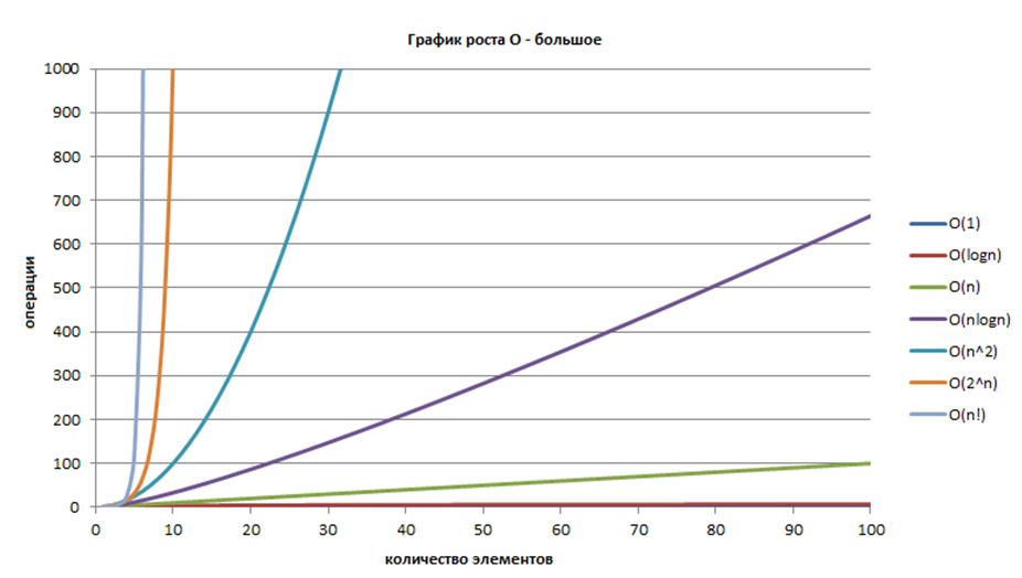
Рисунок 6.1.1 — График роста \(O\) -большое 6 ¶

6.1.3. Оценка сложности алгоритмов¶

Для оценки вычислительной сложности алгоритмов необходимо знать и учитывать сложности:

используемых структур данных;

совокупности различных операций.

6.1.3.1. Операции над структурами данных¶

В Python имеются коллекции (структуры данных), операции над которыми имеют определенную сложность.

6.1.3.1.1. Список и кортеж¶

Большинство операций со списком/кортежем имеют сложность \(O(N)\) (Таблица 6.1.1).

Таблица 6.1.1 — Асимптотические сложности для списка или кортежа ¶