Запуск надстройки Power Pivot для Excel
Power Pivot — это надстройка, с помощью которую можно выполнять мощный анализ данных в Excel. Надстройка встроена в определенные версии Office, но по умолчанию не включена.
Список версий Office, которые включают Power Pivot, а также список версий, в которых их нет, см. в вопросе Где Power Pivot?
Вот как можно включить Power Pivot перед первым использованием.
Перейдите на вкладку Файл > Параметры > Надстройки.
В поле Управление выберите Надстройки COM и нажмите Перейти.
Установите флажок Microsoft Office Power Pivot и нажмите кнопку ОК. Если установлены другие версии Power Pivot, то они будут также перечислены в списке надстроек COM. Выберите надстройку Power Pivot для Excel.
На ленте появится вкладка Power Pivot.

Откройте окно Power Pivot.
Щелкните Power Pivot.
На этой вкладке можно работать со сводными таблицами, вычисляемыми полями и ключевыми показателями эффективности Power Pivot, а также создавать связанные таблицы.
Нажмите кнопку Управление.

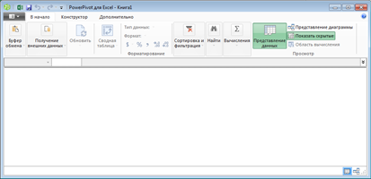
Откроется окно Power Pivot. Здесь вы можете нажать кнопку «Внешние данные», чтобы использовать мастер импорта таблиц для фильтрации данных при их добавлении в файл, создания связей между таблицами, обогащения данных вычислениями и выражениями и создании сводных таблиц и сводных диаграмм на их основе.
Устранение неполадок: исчезновение ленты Power Pivot
В редких случаях лента Power Pivot исчезает из меню, когда Excel определяет, что надстройка нарушает его работу. Это может произойти, если Excel неожиданно завершает работу при открытом окне Power Pivot. Чтобы восстановить меню Power Pivot:
Выберите Файл > Параметры > Надстройки.
В поле Управление выберите Отключенные объекты > Перейти.
Выберите Microsoft OfficePower Pivot и нажмите кнопку Включить.
Если не удается восстановить ленту Power Pivot, выполнив указанные выше действия, или лента исчезает, когда вы закрываете и снова открываете Excel, сделайте следующее:
откройте меню Пуск > Выполнить и введите команду regedit;
В редакторе реестра разверните следующий раздел:
Для Excel 2013: HKEY_CURRENT_USER > Software > Microsoft > Office > 15.0 > User Settings.
Для Excel 2016: HKEY_CURRENT_USER > Software > Microsoft > Office > 16.0 > User Settings
щелкните правой кнопкой мыши PowerPivotExcelAddin, а затем нажмите Удалить;
вернитесь в верхнюю часть редактора реестра;
разверните раздел HKEY_CURRENT_USER > Software > Microsoft > Office > Excel > Addins;
Enabling Power Pivot Excel 2016
Power Pivot is an Excel add-in that was first introduced in Excel 2010 by Microsoft. It allows you to harness the power of Business Intelligence right in Excel.
In this tutorial, you will be provided with a detailed guide on
- What is Power Pivot?
- How to open the Power Pivot window?
Let’s go through each point one-by-one!
What is Power Pivot?
Power Pivot gives you the power to work with large sets of data.
In a nutshell, it allows you to use multiple data sources. Then you could import, merge and perform analysis on the resulting data.
The beautiful thing with Power Pivot is it allows you to work on Big Data with no limitations.
Imagine getting data from multiple sources like SQL Server, Oracle, XML, Excel, Microsoft Access then build a Data Model from it. Then you can analyze these all into one awesome Pivot Table!
How to Enable Power Pivot for Excel 2016?
So how do I get my hands on this super awesome add-in…I hear you say?
The good thing with Power Pivot is it already comes with your Excel 2016, we need to enable it to start using Power Pivot.
You just need to make sure you have one of these versions:
Power Pivot is NOT AVAILABLE in Office 2016 for the following products:
Office 365 Home, Office 365 Personal, Office 365 Business Essentials, Office 365 Business, Office 365 Business Premium, Office 365 Enterprise E1
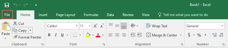
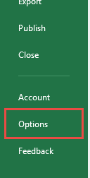
STEP 1 : Go to File > Options
STEP 2: Go to Add-Ins, for the Manage dropdown select COM Add-ins. Click Go once set.
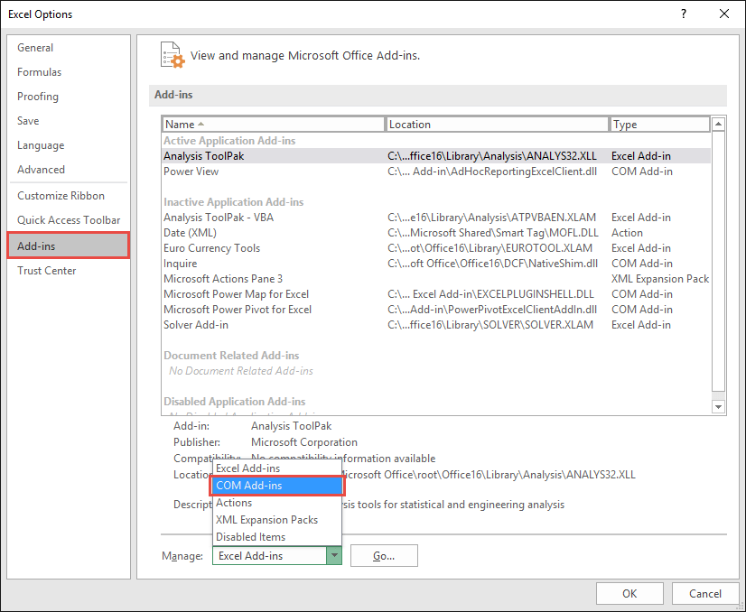
STEP 3: Check Microsoft Power Pivot for Excel. Click OK once done.
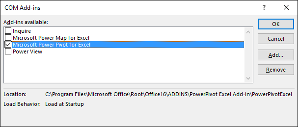
You can easily enable Pivot Excel 2016 download and make the tab appear in the menu ribbon.
STEP 4: You should now have the Power Pivot Tab. Click Manage to see the Power Pivot Window.
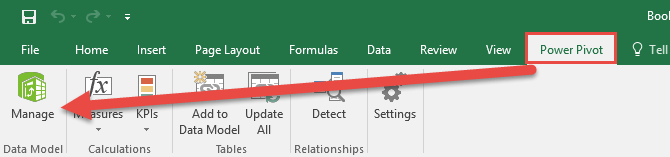
This will open Power Pivot in Excel 2016!
Power Pivot Window (click on the image to expand):

Getting Started with Power Pivot Excel 2016
To work on Power Pivot, you must first understand how to open the Power Pivot window.
How to open the Power Pivot window?
STEP 1: Click on the Power Pivot Tab in Menu Ribbon.

STEP 2: Select the Manage option under Data Model.

This opens the Power Pivot window and here you can explore all of its features!
Adding Data to Data Model
The first step is to add some data to your model. You can import data from two categories:
- From the Current Workbook
- From External Data Sources.
Let’s talk about each one of them in detail.
To Import data from the Current Workbook, follow the steps below:
STEP 1: Highlight the Data in your current workbook.
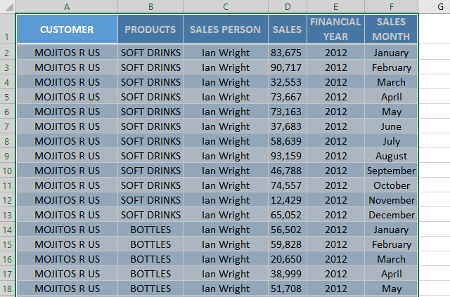
STEP 2: Go to Insert > Table to convert data into a table.

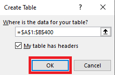
STEP 3: In the Create Table dialog box, Click OK.
STEP 4: Go to Power Pivot > Add to Data Model.

This will import the data into the power pivot window.
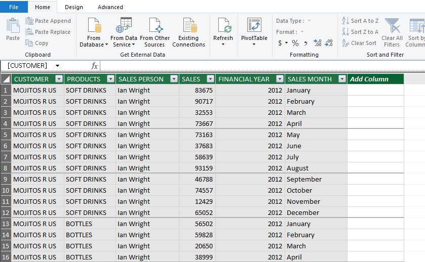
To Import data from an External Data Source like an Excel File, follow the step-by-step tutorial below:
STEP 1: Click on Power Pivot > Manage to open the Power Pivot Window.
STEP 2: Click on Home > From Other Sources.

STEP 3: In the Table Import Wizard, Select Excel File and Click Next.
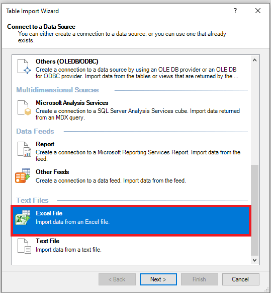
STEP 4: Click on Browse.
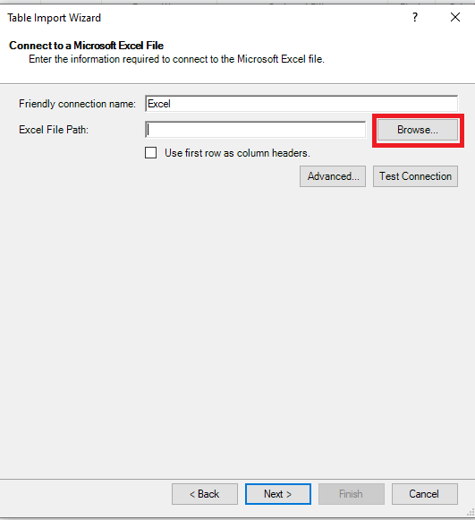
STEP 5: Select the Excel file that you want to import.
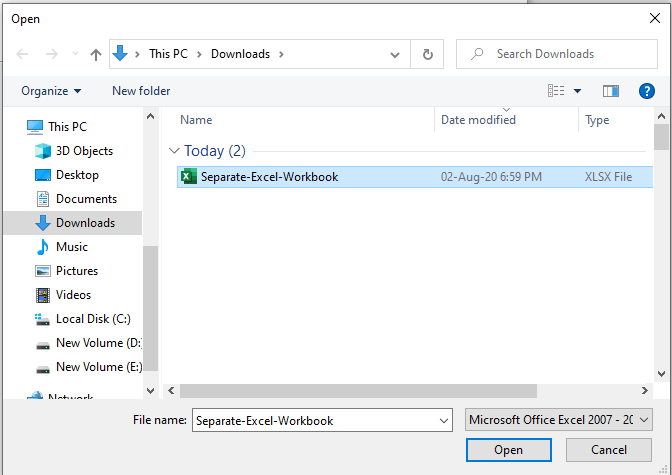
STEP 6: Click Next. Make sure to check the box for Use first row as column headers.
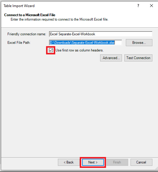
STEP 7: Click Next (As the desired sheet is already selected here)
If you have multiple sheets in your file, it will be displayed here and you can select the one you want to import.
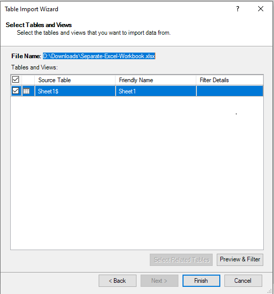
If you also apply a filter in your data as per your required. Say, you want to display data for the month of January, February, and April only.
You can do that by clicking on the Preview & Filter button and then applying the filter.
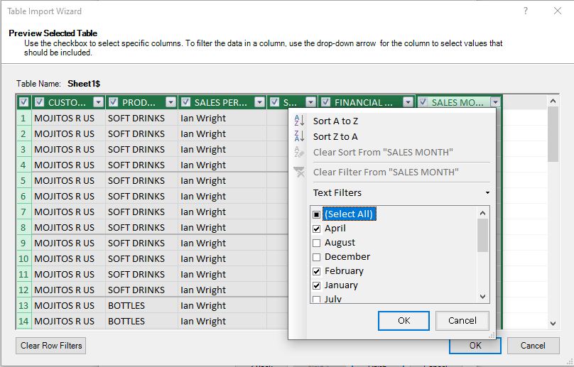
Only the filtered data will be imported to Power Pivot.
STEP 8: Click Finish.
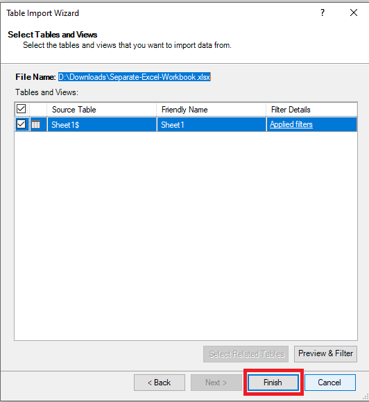
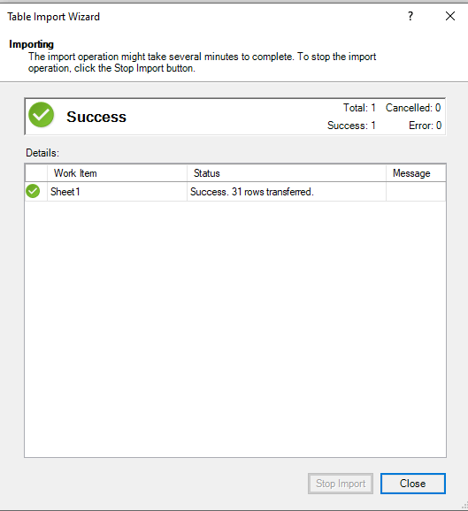
STEP 9: A Success message will be displayed showing you the number of rows that have been imported. Verify that and Click Close.
Different Views in Power Pivot
There are two views that are available in Power Pivot – Data View and Diagram View.
Data View
This is the view shown to Excel users by default.
Data view displays a table of your data model in a grid format, much like the standard Excel. Each table has its own tab at the bottom of the sheet. You cannot make any edits in the cells in the data view.
A data view is comprised of two parts – the Table area and the Calculation area.
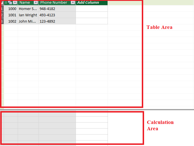
The Table area is where the data table is displayed and the Calculation area is just below the table area where you can create measures.
You can even hide the Calculation area if it is not required by clicking on the Home > Calculation Area.

Diagram View
Ever faced a situation when you have multiple tables in Power Pivot and you are unable to analyze the relationship?
Diagram View provides a perfect solution for this problem – a bird’s eye view for all your tables.
Let’s look at an example of how data is displayed in Diagram View.
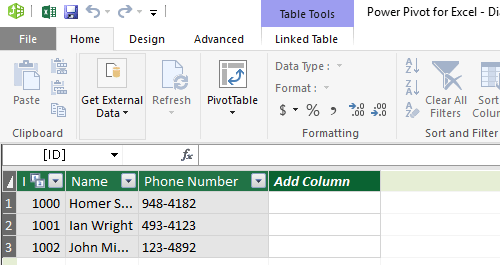
You have two tables – Names and Sales.
Names Table
Sales Table
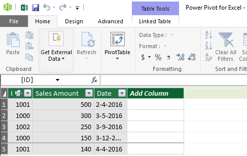
The ID column of the Sales Table is linked to the ID column of the Name Table.
*** You can view the exact step-by-step tutorial of how this was done here: Linking Excel Tables in Power Pivot. ***
To get a bird’s eye view of this relationship, Go to Home > Diagram View
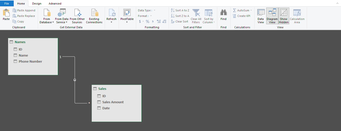
In Diagram View, each table is represented using a box with the header as table name, and then below is the name of the columns of that particular table.
You can drag the corner of the table to resize them and can also move them to different locations.
Create Relationship in Power Pivot
In the example above, you have imported the two tables in the Power Pivot window. You can now link the ID column from the Names table with the ID column in Sales Table.
Let’s see how it can be done by following the steps below:
STEP 1: In the Power Pivot window, Go to Home > Diagram View.

STEP 2: Select the Column Heading and drag to connect it to the Column heading of the second table.
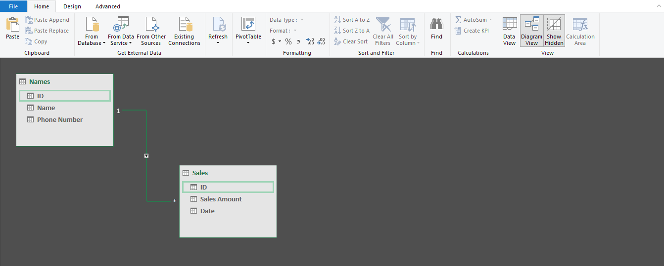
To view the relationship created, simply double click on the arrow linking the two tables.
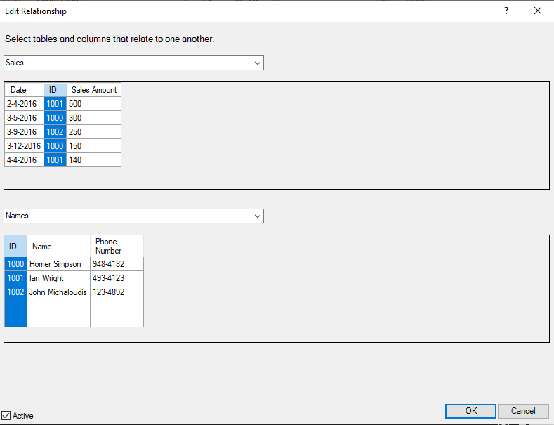
As you can see the ID column is highlighted in both the tables indicating the link between the two columns.
Create Pivot Table using Power Pivot data
STEP 1: Click on the Power Pivot Tab in Menu Ribbon.
STEP 2: Select the Manage option under Data Model.
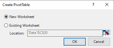
STEP 3: In the Power Pivot window, Go to Home > PivotTable.

STEP 4: In the Create PowerTable dialog box, Select New Worksheet and click OK.
STEP 5: In the PivotTable Fields panel, you can drag and drop fields to create a customized PivotTable.
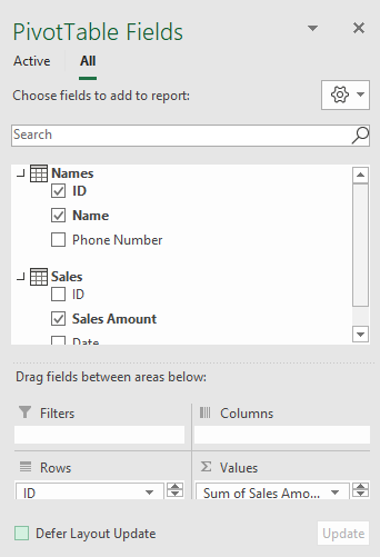
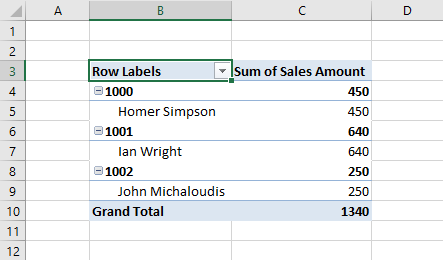
This is how the PivotTable will look like:
Advantages of using Power Pivot Excel 2016
The main advantages of using Power Pivot Excel 2016 are as follows:
- You can work with millions of rows and extract data from multiple sources.
- You can process calculations and analysis faster.
- You can import data from multiple sources and you can also filter data and rename columns while importing.
- When you import a table in Power Pivot, each table gets organized in individual tabbed pages.
- You can create your own formula using DAX expression.
- You can create relationships among the table to easily analyze data fields together.
- You can create calculated fields and calculated columns in the data table.
Conclusion
In this article, you have learned about Power Pivot Excel 2016 download- how to install Power Pivot for Excel 2016, Open a power pivot window, add data to model from current file or external sources, different views in power pivot excel 2016, and lastly the advantages of using Power Pivot.
There is a lot you can do using this tool. Click here to learn more.
You can learn more about how to use Excel by viewing our FREE Excel webinar training on Formulas, Pivot Tables, and Macros & VBA!
Как установить power pivot в excel 2016
Hi, as powerpivot is not a part of excel 2016 standard version and available in professional version only. Therefore, I want to know that how can I install or add this feature on my standard version.
Previously I was using excel 2010 standard version and powerpivot download is available on microsoft website for this version.
Now, I’ve upgraded the same into 2016 and I’m unable to use it.
Please help me out.
All replies
Unfortunately, PowerPivot is not available in Excel 2016 Standard version, it is available in:
Office Professional Plus 2016 and Office Professional.
Office 2016 Standalone
Microsoft Office 365 ProPlus available as a standalone subscription.
Microsoft Office 365 ProPlus available as part of the Office 365 Enterprise E3, Office 365 Enterprise E4, Office 365 Education E2, Office 365 Education E3, Office 365 Government E3, or Office 365 Government E4 offerings.There isn’t any ways to download and install PowerPivot for Excel Standard 2016.
Hope the information was helpful. Anything unclear, feel free to post back to let us know.
Please remember to mark the replies as answers if they helped. If you have feedback for TechNet Subscriber Support, contact tnsf@microsoft.com.
Click here to learn more. Visit the dedicated forum to share, explore and talk to experts about Microsoft Office 2019.
Exceltip
Блог о программе Microsoft Excel: приемы, хитрости, секреты, трюки
Загрузка и установка PowerPivot
В данной статье мы расскажем о процессе установки PowerPivot для Excel и познакомим с основными элементами данной надстройки.
Системные требования
Чтобы установить PowerPivot для Excel вам понадобиться 32-х или 64-х битная версия Excel 2010 и старше, работающая на операционной системе Windows.
Для загрузки надстройки PowerPivot доступны две версии: 32-х и 64-х битная.
Если вы не уверены, какая разрядность у вашей версии, зайдите в Excel, перейдите по вкладке Файл -> Учетная запись –> О программе Excel. В появившемся диалоговом окне, вы найдете интересующую вас информацию.

Установка PowerPivot
Для Excel 2010, необходимо скачать пакет установки с официального сайта Microsoft.
Убедитесь, что все Office программы закрыты и запустите установщик. Через несколько минут установка завершится. При первом запуске Excel, вы увидите краткое уведомление, что Microsoft регистрирует PowerPivot. В последующие запуски вы не заметите никакой задержки связанной с надстройкой.
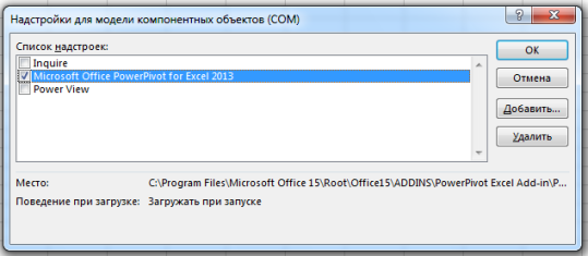
Для Excel 2013 ничего скачивать не надо, так как он уже содержит PowerPivot в своей комплектации. Перейдите по вкладке Файл –> Параметры –> Надстройки. В диалоговом окне выберите Надстройки COM –> Перейти. В появившемся окне поставьте галочку напротив Microsoft Office PowerPivot for Excel 2013 и нажмите OK.
Вкладка PowerPivot
После установки на ленте справа вы увидите новую вкладку PowerPivot, которая содержит необычный набор иконок. Некоторые из них продублированы в приложении PowerPivot.
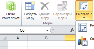

Окно PowerPivot. Вызывает приложение PowerPivot.
Создать меру. После того, как вы создадите сводную таблицу, у вас появится возможность воспользоваться языком формул DAX для создания вычисляемого поля. В PowerPivot такие поля называются мерой.
Создание связанной таблицы. Есть два пути получения данных с листа Excel в PowerPivot. Первый, копирование и вставка данных для обработки в приложении. Второй, создание связи с реальной таблицей. Для этих целей вам и понадобится эта икнока.
Список полей. Список полей для PowerPivot не совсем такой же, как для сводных таблиц. Команда разработчиков превратила список полей OLAP в более дружественный вид PowerPivot. Вы можете скрывать его с помощью этой иконки.
Обнаружение связей. Этот переключатель позволяет автоматически обнаруживать связи между таблицами.
Вкладки окна PowerPivot
Когда вы щелкните по кнопке Окно PowerPivot, находящееся в левой части ленты, вы попадете в приложение PowerPivot, которое будет иметь 4 вкладки ленты.
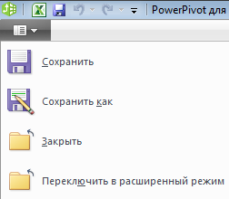
Файл. Тут вы найдете Сохранить, Сохранить как, Закрыть и Переключиться в обычный режим
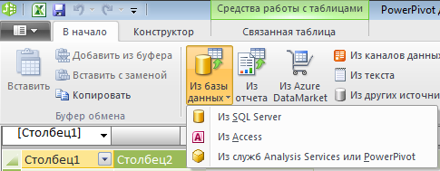
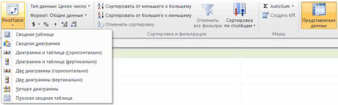
В начало. Здесь находятся инструменты импорта данных в PowerPivot, создания сводных таблиц и инструменты фильтрации и сортировки.
Конструктор. Инструменты управления отношениями между таблицами.
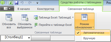
Связанные таблицы. Инструменты управления ссылками с листа Excel.
Использование вкладки Файл
Все пункты вкладки Файл связаны с Excel. Щелчок на Сохранить как вернет вас в Excel и откроет диалоговое окно сохранения. Щелчок на Закрыть просто вернет вас в Excel.
Использование вкладки В начало
В правой части вкладки В начало находятся инструменты, связанные с импортом данных в PowerPivot. Вы можете воспользоваться буфером обмена, чтобы вставить новую таблицу, либо добавить или заменить строки в уже существующей. Вы также можете импортировать данные с баз данных, из отчета SharePoint, из канала данных ATOM или текстового файла.
В правой части вкладки В начало находятся инструменты связанные с отображением данных в окне PowerPivot.
Использование вкладки Конструктор
Во вкладке Конструктор вы сможете добавить новые колонки или создать связи между таблицами. К тому же в данной вкладке можно вводить формулы DAX и создавать вычисляемы столбцы.

Использование вкладки Связанные таблицы
Данная вкладка доступна только тогда, когда у вас есть связанная с Excel таблица. Здесь вы можете воспользоваться иконками для обновления данных, либо для переключения режимов обновления: автоматический или ручной.
Вам также могут быть интересны следующие статьи
Один комментарий
как вы сказали я сделал: зашел в надстройки потом в настройки COM но там нет PowerPivot только Power Query , хоть у меня 2013 excel 64-х разрядный ,что делать?