statistics — Mathematical statistics functions
This module provides functions for calculating mathematical statistics of numeric ( Real -valued) data.
The module is not intended to be a competitor to third-party libraries such as NumPy, SciPy, or proprietary full-featured statistics packages aimed at professional statisticians such as Minitab, SAS and Matlab. It is aimed at the level of graphing and scientific calculators.
Unless explicitly noted, these functions support int , float , Decimal and Fraction . Behaviour with other types (whether in the numeric tower or not) is currently unsupported. Collections with a mix of types are also undefined and implementation-dependent. If your input data consists of mixed types, you may be able to use map() to ensure a consistent result, for example: map(float, input_data) .
Some datasets use NaN (not a number) values to represent missing data. Since NaNs have unusual comparison semantics, they cause surprising or undefined behaviors in the statistics functions that sort data or that count occurrences. The functions affected are median() , median_low() , median_high() , median_grouped() , mode() , multimode() , and quantiles() . The NaN values should be stripped before calling these functions:
Averages and measures of central location
These functions calculate an average or typical value from a population or sample.
Arithmetic mean (“average”) of data.
Fast, floating point arithmetic mean, with optional weighting.
Geometric mean of data.
Harmonic mean of data.
Median (middle value) of data.
Low median of data.
High median of data.
Median, or 50th percentile, of grouped data.
Single mode (most common value) of discrete or nominal data.
List of modes (most common values) of discrete or nominal data.
Divide data into intervals with equal probability.
Measures of spread
These functions calculate a measure of how much the population or sample tends to deviate from the typical or average values.
Population standard deviation of data.
Population variance of data.
Sample standard deviation of data.
Sample variance of data.
Statistics for relations between two inputs
These functions calculate statistics regarding relations between two inputs.
Sample covariance for two variables.
Pearson’s correlation coefficient for two variables.
Slope and intercept for simple linear regression.
Function details
Note: The functions do not require the data given to them to be sorted. However, for reading convenience, most of the examples show sorted sequences.
statistics. mean ( data ) 
Return the sample arithmetic mean of data which can be a sequence or iterable.
The arithmetic mean is the sum of the data divided by the number of data points. It is commonly called “the average”, although it is only one of many different mathematical averages. It is a measure of the central location of the data.
If data is empty, StatisticsError will be raised.
Some examples of use:
The mean is strongly affected by outliers and is not necessarily a typical example of the data points. For a more robust, although less efficient, measure of central tendency, see median() .
The sample mean gives an unbiased estimate of the true population mean, so that when taken on average over all the possible samples, mean(sample) converges on the true mean of the entire population. If data represents the entire population rather than a sample, then mean(data) is equivalent to calculating the true population mean μ.
Convert data to floats and compute the arithmetic mean.
This runs faster than the mean() function and it always returns a float . The data may be a sequence or iterable. If the input dataset is empty, raises a StatisticsError .
Optional weighting is supported. For example, a professor assigns a grade for a course by weighting quizzes at 20%, homework at 20%, a midterm exam at 30%, and a final exam at 30%:
If weights is supplied, it must be the same length as the data or a ValueError will be raised.
New in version 3.8.
Changed in version 3.11: Added support for weights.
Convert data to floats and compute the geometric mean.
The geometric mean indicates the central tendency or typical value of the data using the product of the values (as opposed to the arithmetic mean which uses their sum).
Raises a StatisticsError if the input dataset is empty, if it contains a zero, or if it contains a negative value. The data may be a sequence or iterable.
No special efforts are made to achieve exact results. (However, this may change in the future.)
New in version 3.8.
Return the harmonic mean of data, a sequence or iterable of real-valued numbers. If weights is omitted or None, then equal weighting is assumed.
The harmonic mean is the reciprocal of the arithmetic mean() of the reciprocals of the data. For example, the harmonic mean of three values a, b and c will be equivalent to 3/(1/a + 1/b + 1/c) . If one of the values is zero, the result will be zero.
The harmonic mean is a type of average, a measure of the central location of the data. It is often appropriate when averaging ratios or rates, for example speeds.
Suppose a car travels 10 km at 40 km/hr, then another 10 km at 60 km/hr. What is the average speed?
Suppose a car travels 40 km/hr for 5 km, and when traffic clears, speeds-up to 60 km/hr for the remaining 30 km of the journey. What is the average speed?
StatisticsError is raised if data is empty, any element is less than zero, or if the weighted sum isn’t positive.
The current algorithm has an early-out when it encounters a zero in the input. This means that the subsequent inputs are not tested for validity. (This behavior may change in the future.)
New in version 3.6.
Changed in version 3.10: Added support for weights.
Return the median (middle value) of numeric data, using the common “mean of middle two” method. If data is empty, StatisticsError is raised. data can be a sequence or iterable.
The median is a robust measure of central location and is less affected by the presence of outliers. When the number of data points is odd, the middle data point is returned:
When the number of data points is even, the median is interpolated by taking the average of the two middle values:
This is suited for when your data is discrete, and you don’t mind that the median may not be an actual data point.
If the data is ordinal (supports order operations) but not numeric (doesn’t support addition), consider using median_low() or median_high() instead.
statistics. median_low ( data ) 
Return the low median of numeric data. If data is empty, StatisticsError is raised. data can be a sequence or iterable.
The low median is always a member of the data set. When the number of data points is odd, the middle value is returned. When it is even, the smaller of the two middle values is returned.
Use the low median when your data are discrete and you prefer the median to be an actual data point rather than interpolated.
statistics. median_high ( data ) 
Return the high median of data. If data is empty, StatisticsError is raised. data can be a sequence or iterable.
The high median is always a member of the data set. When the number of data points is odd, the middle value is returned. When it is even, the larger of the two middle values is returned.
Use the high median when your data are discrete and you prefer the median to be an actual data point rather than interpolated.
statistics. median_grouped ( data , interval = 1 ) 
Return the median of grouped continuous data, calculated as the 50th percentile, using interpolation. If data is empty, StatisticsError is raised. data can be a sequence or iterable.
In the following example, the data are rounded, so that each value represents the midpoint of data classes, e.g. 1 is the midpoint of the class 0.5–1.5, 2 is the midpoint of 1.5–2.5, 3 is the midpoint of 2.5–3.5, etc. With the data given, the middle value falls somewhere in the class 3.5–4.5, and interpolation is used to estimate it:
Optional argument interval represents the class interval, and defaults to 1. Changing the class interval naturally will change the interpolation:
This function does not check whether the data points are at least interval apart.
CPython implementation detail: Under some circumstances, median_grouped() may coerce data points to floats. This behaviour is likely to change in the future.
“Statistics for the Behavioral Sciences”, Frederick J Gravetter and Larry B Wallnau (8th Edition).
The SSMEDIAN function in the Gnome Gnumeric spreadsheet, including this discussion.
Return the single most common data point from discrete or nominal data. The mode (when it exists) is the most typical value and serves as a measure of central location.
If there are multiple modes with the same frequency, returns the first one encountered in the data. If the smallest or largest of those is desired instead, use min(multimode(data)) or max(multimode(data)) . If the input data is empty, StatisticsError is raised.
mode assumes discrete data and returns a single value. This is the standard treatment of the mode as commonly taught in schools:
The mode is unique in that it is the only statistic in this package that also applies to nominal (non-numeric) data:
Changed in version 3.8: Now handles multimodal datasets by returning the first mode encountered. Formerly, it raised StatisticsError when more than one mode was found.
Return a list of the most frequently occurring values in the order they were first encountered in the data. Will return more than one result if there are multiple modes or an empty list if the data is empty:
New in version 3.8.
Return the population standard deviation (the square root of the population variance). See pvariance() for arguments and other details.
Return the population variance of data, a non-empty sequence or iterable of real-valued numbers. Variance, or second moment about the mean, is a measure of the variability (spread or dispersion) of data. A large variance indicates that the data is spread out; a small variance indicates it is clustered closely around the mean.
If the optional second argument mu is given, it is typically the mean of the data. It can also be used to compute the second moment around a point that is not the mean. If it is missing or None (the default), the arithmetic mean is automatically calculated.
Use this function to calculate the variance from the entire population. To estimate the variance from a sample, the variance() function is usually a better choice.
If you have already calculated the mean of your data, you can pass it as the optional second argument mu to avoid recalculation:
Decimals and Fractions are supported:
When called with the entire population, this gives the population variance σ². When called on a sample instead, this is the biased sample variance s², also known as variance with N degrees of freedom.
If you somehow know the true population mean μ, you may use this function to calculate the variance of a sample, giving the known population mean as the second argument. Provided the data points are a random sample of the population, the result will be an unbiased estimate of the population variance.
Return the sample standard deviation (the square root of the sample variance). See variance() for arguments and other details.
Return the sample variance of data, an iterable of at least two real-valued numbers. Variance, or second moment about the mean, is a measure of the variability (spread or dispersion) of data. A large variance indicates that the data is spread out; a small variance indicates it is clustered closely around the mean.
If the optional second argument xbar is given, it should be the mean of data. If it is missing or None (the default), the mean is automatically calculated.
Use this function when your data is a sample from a population. To calculate the variance from the entire population, see pvariance() .
Raises StatisticsError if data has fewer than two values.
If you have already calculated the mean of your data, you can pass it as the optional second argument xbar to avoid recalculation:
This function does not attempt to verify that you have passed the actual mean as xbar. Using arbitrary values for xbar can lead to invalid or impossible results.
Decimal and Fraction values are supported:
This is the sample variance s² with Bessel’s correction, also known as variance with N-1 degrees of freedom. Provided that the data points are representative (e.g. independent and identically distributed), the result should be an unbiased estimate of the true population variance.
If you somehow know the actual population mean μ you should pass it to the pvariance() function as the mu parameter to get the variance of a sample.
Divide data into n continuous intervals with equal probability. Returns a list of n — 1 cut points separating the intervals.
Set n to 4 for quartiles (the default). Set n to 10 for deciles. Set n to 100 for percentiles which gives the 99 cuts points that separate data into 100 equal sized groups. Raises StatisticsError if n is not least 1.
The data can be any iterable containing sample data. For meaningful results, the number of data points in data should be larger than n. Raises StatisticsError if there are not at least two data points.
The cut points are linearly interpolated from the two nearest data points. For example, if a cut point falls one-third of the distance between two sample values, 100 and 112 , the cut-point will evaluate to 104 .
The method for computing quantiles can be varied depending on whether the data includes or excludes the lowest and highest possible values from the population.
The default method is “exclusive” and is used for data sampled from a population that can have more extreme values than found in the samples. The portion of the population falling below the i-th of m sorted data points is computed as i / (m + 1) . Given nine sample values, the method sorts them and assigns the following percentiles: 10%, 20%, 30%, 40%, 50%, 60%, 70%, 80%, 90%.
Setting the method to “inclusive” is used for describing population data or for samples that are known to include the most extreme values from the population. The minimum value in data is treated as the 0th percentile and the maximum value is treated as the 100th percentile. The portion of the population falling below the i-th of m sorted data points is computed as (i — 1) / (m — 1) . Given 11 sample values, the method sorts them and assigns the following percentiles: 0%, 10%, 20%, 30%, 40%, 50%, 60%, 70%, 80%, 90%, 100%.
New in version 3.8.
Return the sample covariance of two inputs x and y. Covariance is a measure of the joint variability of two inputs.
Both inputs must be of the same length (no less than two), otherwise StatisticsError is raised.
New in version 3.10.
Return the Pearson’s correlation coefficient for two inputs. Pearson’s correlation coefficient r takes values between -1 and +1. It measures the strength and direction of the linear relationship, where +1 means very strong, positive linear relationship, -1 very strong, negative linear relationship, and 0 no linear relationship.
Both inputs must be of the same length (no less than two), and need not to be constant, otherwise StatisticsError is raised.
New in version 3.10.
Return the slope and intercept of simple linear regression parameters estimated using ordinary least squares. Simple linear regression describes the relationship between an independent variable x and a dependent variable y in terms of this linear function:
y = slope * x + intercept + noise
where slope and intercept are the regression parameters that are estimated, and noise represents the variability of the data that was not explained by the linear regression (it is equal to the difference between predicted and actual values of the dependent variable).
Both inputs must be of the same length (no less than two), and the independent variable x cannot be constant; otherwise a StatisticsError is raised.
For example, we can use the release dates of the Monty Python films to predict the cumulative number of Monty Python films that would have been produced by 2019 assuming that they had kept the pace.
If proportional is true, the independent variable x and the dependent variable y are assumed to be directly proportional. The data is fit to a line passing through the origin. Since the intercept will always be 0.0, the underlying linear function simplifies to:
y = slope * x + noise
New in version 3.10.
Changed in version 3.11: Added support for proportional.
Exceptions
A single exception is defined:
exception statistics. StatisticsError 
Subclass of ValueError for statistics-related exceptions.
NormalDist objects
NormalDist is a tool for creating and manipulating normal distributions of a random variable. It is a class that treats the mean and standard deviation of data measurements as a single entity.
Normal distributions arise from the Central Limit Theorem and have a wide range of applications in statistics.
class statistics. NormalDist ( mu = 0.0 , sigma = 1.0 ) 
Returns a new NormalDist object where mu represents the arithmetic mean and sigma represents the standard deviation.
A read-only property for the arithmetic mean of a normal distribution.
A read-only property for the median of a normal distribution.
A read-only property for the mode of a normal distribution.
A read-only property for the standard deviation of a normal distribution.
A read-only property for the variance of a normal distribution. Equal to the square of the standard deviation.
classmethod from_samples ( data ) 
Makes a normal distribution instance with mu and sigma parameters estimated from the data using fmean() and stdev() .
The data can be any iterable and should consist of values that can be converted to type float . If data does not contain at least two elements, raises StatisticsError because it takes at least one point to estimate a central value and at least two points to estimate dispersion.
Generates n random samples for a given mean and standard deviation. Returns a list of float values.
If seed is given, creates a new instance of the underlying random number generator. This is useful for creating reproducible results, even in a multi-threading context.
Using a probability density function (pdf), compute the relative likelihood that a random variable X will be near the given value x. Mathematically, it is the limit of the ratio P(x <= X < x+dx) / dx as dx approaches zero.
The relative likelihood is computed as the probability of a sample occurring in a narrow range divided by the width of the range (hence the word “density”). Since the likelihood is relative to other points, its value can be greater than 1.0 .
Using a cumulative distribution function (cdf), compute the probability that a random variable X will be less than or equal to x. Mathematically, it is written P(X <= x) .
Compute the inverse cumulative distribution function, also known as the quantile function or the percent-point function. Mathematically, it is written x : P(X <= x) = p .
Finds the value x of the random variable X such that the probability of the variable being less than or equal to that value equals the given probability p.
Measures the agreement between two normal probability distributions. Returns a value between 0.0 and 1.0 giving the overlapping area for the two probability density functions.
Divide the normal distribution into n continuous intervals with equal probability. Returns a list of (n — 1) cut points separating the intervals.
Set n to 4 for quartiles (the default). Set n to 10 for deciles. Set n to 100 for percentiles which gives the 99 cuts points that separate the normal distribution into 100 equal sized groups.
Compute the Standard Score describing x in terms of the number of standard deviations above or below the mean of the normal distribution: (x — mean) / stdev .
New in version 3.9.
Instances of NormalDist support addition, subtraction, multiplication and division by a constant. These operations are used for translation and scaling. For example:
Dividing a constant by an instance of NormalDist is not supported because the result wouldn’t be normally distributed.
Since normal distributions arise from additive effects of independent variables, it is possible to add and subtract two independent normally distributed random variables represented as instances of NormalDist . For example:
New in version 3.8.
NormalDist Examples and Recipes
NormalDist readily solves classic probability problems.
For example, given historical data for SAT exams showing that scores are normally distributed with a mean of 1060 and a standard deviation of 195, determine the percentage of students with test scores between 1100 and 1200, after rounding to the nearest whole number:
Find the quartiles and deciles for the SAT scores:
To estimate the distribution for a model than isn’t easy to solve analytically, NormalDist can generate input samples for a Monte Carlo simulation:
Normal distributions can be used to approximate Binomial distributions when the sample size is large and when the probability of a successful trial is near 50%.
For example, an open source conference has 750 attendees and two rooms with a 500 person capacity. There is a talk about Python and another about Ruby. In previous conferences, 65% of the attendees preferred to listen to Python talks. Assuming the population preferences haven’t changed, what is the probability that the Python room will stay within its capacity limits?
Normal distributions commonly arise in machine learning problems.
Wikipedia has a nice example of a Naive Bayesian Classifier. The challenge is to predict a person’s gender from measurements of normally distributed features including height, weight, and foot size.
We’re given a training dataset with measurements for eight people. The measurements are assumed to be normally distributed, so we summarize the data with NormalDist :
Next, we encounter a new person whose feature measurements are known but whose gender is unknown:
Starting with a 50% prior probability of being male or female, we compute the posterior as the prior times the product of likelihoods for the feature measurements given the gender:
The final prediction goes to the largest posterior. This is known as the maximum a posteriori or MAP:
mode() function in Python statistics module
The mode of a set of data values is the value that appears most often. It is the value at which the data is most likely to be sampled. A mode of a continuous probability distribution is often considered to be any value x at which its probability density function has a local maximum value, so any peak is a mode.
Python is very robust when it comes to statistics and working with a set of a large range of values. The statistics module has a very large number of functions to work with very large data-sets. The mode() function is one of such methods. This function returns the robust measure of a central data point in a given range of data-sets.
Example :
Code #1 : This piece will demonstrate mode() function through a simple example.
Mean, mode, median, deviation and quantiles in Python

Quick explanation and Python examples on how to calculate most popular statistical metrics for data analysis. We’re going to use awesome Numpy package for our examples.
Mean is an average of all values in the dataset:
Median
Median, on the contrary, is the value which divides the whole dataset into 2 sets of values:
To calculate median, we should first sort our dataset, then divide it into 2 sets, and then pick value which is in the center of 2 sets:
- If we have odd number of values in original set, we just sort the set and pick central value.
- If we have even number of values, we should calculate average of 2 central values after sorting.
Median is better than average, as “strange” values (like 40 in our case) will have less impact on the resulting value:
At the same time, median value better describes point, which most values are distributed around.
Mode shows the most popular value in the dataset:
Unfortunately Numpy lacks mode calculation, but it can be done using scipy package.
Quantiles
Quantile is a way to say how many values in original dataset is less than certain level:
So 0.75 quantile (the same as 75% percentile) is a smallest value which is bigger than 75% of the smallest values from dataset. Most popular quantiles are 0.25, .50 and .75:
As you can see, 0.50 quantile (or 50% percentile) is the same as median.
Deviation
Deviation allows to evaluate how values are far from each other. In other words — how big values spread is. Most popular method for calculating deviation is based on values distance from average:
If we calculate all distances, then sum their squares (in order to make all values positive) and divide by number of values in dataset, we get square of standard deviation:
Python, исследование данных и выборы: часть 2
Пост №2 для начинающих посвящен описательным статистикам, группированию данных и нормальному распределению. Все эти сведения заложат основу для дальнейшего анализа электоральных данных. Предыдущий пост см. здесь.
Описательные статистики
Описательные статистические величины, или статистики, — это числа, которые используются для обобщения и описания данных. В целях демонстрации того, что мы имеем в виду, посмотрим на столбец с данными об электорате Electorate. Он показывает суммарное число зарегистрированных избирателей в каждом избирательном округе:
Мы уже очистили столбец, отфильтровав пустые значения ( nan ) из набора данных, и поэтому предыдущий пример должен вернуть суммарное число избирательных округов.
Описательные статистики, так называемые сводные статистики, представляют собой разные подходы к измерению свойств последовательностей чисел. Они помогают охарактеризовать последовательность и способны выступать в качестве ориентира для дальнейшего анализа. Начнем с двух самых базовых статистик, которые мы можем вычислить из последовательности чисел — ее среднее значение и дисперсию (варианс).
Среднее значение
Наиболее распространенный способ усреднить набор данных — взять его среднее значение. Среднее значение на самом деле представляет собой один из нескольких способов измерения центра распределения данных.
Среднее значение числового ряда вычисляется на Python следующим образом:
Мы можем воспользоваться нашей новой функцией mean для вычисления среднего числа избирателей в Великобритании:
На самом деле, библиотека pandas уже содержит функцию mean, которая гораздо эффективнее вычисляет среднее значение последовательности. В нашем случае ее можно применить следующим образом:
Медиана
Медиана — это еще одна распространенная описательная статистика для измерения центра распределения последовательности. Если Вы упорядочили все данные от меньшего до наибольшего, то медиана — это значение, которое находится ровно по середине. Если в последовательности число точек данных четное, то медиана определяется, как полусумма двух срединных значений.
Медианное значение электората Великобритании составляет:
Библиотека pandas тоже располагает встроенной функцией для вычисления медианного значения, которая так и называется median .
Дисперсия
Среднее арифметическое и медиана являются двумя альтернативными способами описания среднего значения последовательности, но сами по себе они мало что говорят о содержащихся в ней значениях. Например, если известно, что среднее последовательности из девяноста девяти значений равно 50, то мы почти ничего не скажем о том, какого рода значения последовательность содержит.
Она может содержать целые числа от одного до девяноста девяти либо сорок девять нулей и пятьдесят девяносто девяток, а может быть и так, что она девяносто восемь раз содержит отрицательную единицу и одно число 5048, или же вообще все значения могут быть равны 50.
Дисперсия (варианс) последовательности чисел показывает «разброс» данных вокруг среднего значения. К примеру, данные, приведенные выше, имели бы разную дисперсию. На языке математики дисперсия обозначается следующим образом:
где s 2 — это математический символ, который часто используют для обозначения дисперсии.
Для вычисления квадрата выражения используется оператор языка Python возведения в степень ** .
Стандартное отклонение
Поскольку мы взяли средний квадрат отклонения, т.е. получили квадрат отклонения и затем его среднее, то единицы измерения дисперсии (варианса) тоже будут в квадрате, т.е. дисперсия электората Великобритании будет измеряться «людьми в квадрате». Несколько неестественно рассуждать об избирателях в таком виде. Единицу измерения можно привести к более естественному виду, снова обозначающему «людей», путем извлечения квадратного корня из дисперсии (варианса). В результате получим так называемое стандартное отклонение, или среднеквадратичное отклонение:
В библиотеке pandas функции для вычисления дисперсии (варианса) и стандартного отклонения имплементированы соответственно, как var и std . При этом последняя по умолчанию вычисляет несмещенное значение, поэтому, чтобы получить тот же самый результат, нужно применить именованный аргумент ddof=0 , который сообщает, что требуется вычислить смещенное значение стандартного отклонения:
Квантили
Медиана представляет собой один из способов вычислить срединное значение из списка, т.е. находящееся ровно по середине, дисперсия же предоставляет способ измерить разброс данных вокруг среднего значения. Если весь разброс данных представить на шкале от 0 до 1, то значение 0.5 будет медианным.
Для примера рассмотрим следующую ниже последовательность чисел:
Отсортированная последовательность состоит из семи чисел, поэтому медианой является число 21 четвертое в ряду. Его также называют 0.5-квантилем. Мы можем получить более полную картину последовательности чисел, взглянув на 0.0 (нулевой), 0.25, 0.5, 0.75 и 1.0 квантили. Все вместе эти цифры не только показывают медиану, но также обобщают диапазон данных и сообщат о характере распределения чисел внутри него. Они иногда упоминаются в связи с пятичисловой сводкой.
Один из способов составления пятичисловой сводки для данных об электорате Великобритании показан ниже. Квантили можно вычислить непосредственно в pandas при помощи функции quantile . Последовательность требующихся квантилей передается в виде списка.
Когда квантили делят диапазон на четыре равных диапазона, как показано выше, то они называются квартилями. Разница между нижним (0.25) и верхним (0.75) квартилями называется межквартильным размахом, или иногда сокращенно МКР. Аналогично дисперсии (варианса) вокруг среднего значения, межквартильный размах измеряет разброс данных вокруг медианы.
Группирование данных в корзины
В целях развития интуитивного понимания в отношении того, что именно все эти расчеты разброса значений измеряют, мы можем применить метод под названием группировка в частотные корзины (binning). Когда данные имеют непрерывный характер, использование специального словаря для подсчета частот Counter (подобно тому, как он использовался при подсчете количества пустых значений в наборе данных об электорате) становится нецелесообразным, поскольку никакие два значения не могут быть одинаковыми. Между тем, общее представление о структуре данных можно все-равно получить, сгруппировав для этого данные в частотные корзины (bins).
Процедура образования корзин заключается в разбиении диапазона значений на ряд последовательных, равноразмерных и меньших интервалов. Каждое значение в исходном ряду попадает строго в одну корзину. Подсчитав количества точек, попадающих в каждую корзину, мы можем получить представление о разбросе данных:

На приведенном выше рисунке показано 15 значений x, разбитых на 5 равноразмерных корзин. Подсчитав количество точек, попадающих в каждую корзину, мы можем четко увидеть, что большинство точек попадают в корзину по середине, а меньшинство — в корзины по краям. Следующая ниже функция Python nbin позволяет добиться того же самого результата:
Например, мы можем разбить диапазон 0-14 на 5 корзин следующим образом:
После того, как мы разбили значения на корзины, мы можем в очередной раз воспользоваться словарем Counter , чтобы подсчитать количество точек в каждой корзине. В следующем ниже примере мы воспользуемся этим словарем для разбиения данных об электорате Великобритании на пять корзин:
Количество точек в крайних корзинах (0 и 4) значительно ниже, чем в корзинах в середине — количества, судя по всему, растут по направлению к медиане, а затем снова снижаются. В следующем разделе мы займемся визуализацией формы этих количеств.
Гистограммы
Гистограмма — это один из способов визуализации распределения одной последовательности значений. Гистограммы попросту берут непрерывное распределение, разбивают его на корзины, и изображают частоты точек, попадающих в каждую корзину, в виде столбцов. Высота каждого столбца гистограммы показывает количество точек данных, которые содержатся в этой корзине.
Мы уже увидели, каким образом можно выполнить разбиение данных на корзины самостоятельно, однако в библиотеке pandas уже содержится функция hist , которая разбивает данные и визуализирует их в виде гистограммы.
Приведенный выше пример сгенерирует следующий ниже график:
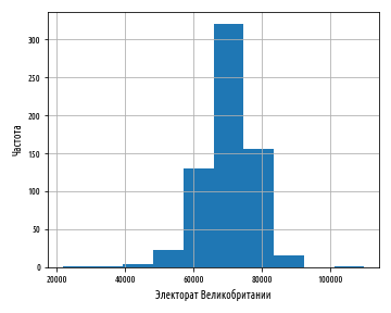
Число корзин, на которые данные разбиваются, можно сконфигурировать, передав в функцию при построении гистограммы именованный аргумент bins :
Приведенный выше график показывает единственный высокий пик, однако он выражает форму данных довольно грубо. Следующий ниже график показывает мелкие детали, но величина столбцов делает неясной форму распределения, в особенности в хвостах:
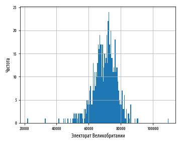
При выборе количества корзин для представления данных следует найти точку равновесия — с малым количеством корзин форма данных будет представлена лишь приблизительно, а слишком большое их число приведет к тому, что шумовые признаки могут заслонить лежащую в основании структуру.
Ниже показана гистограмма теперь уже из 20 корзин:

Окончательный график, состоящий из 20 корзин, судя по всему, пока лучше всего представляет эти данные.
Наряду со средним значением и медианой, есть еще один способ измерить среднюю величину последовательности. Это мода. Мода — это значение, встречающееся в последовательности наиболее часто. Она определена исключительно только для последовательностей, имеющих по меньшей мере одно дублирующее значение; во многих статистических распределениях это не так, и поэтому для них мода не определена. Тем не менее, пик гистограммы часто называют модой, поскольку он соответствует наиболее распространенной корзине.
Из графика ясно видно, что распределение вполне симметрично относительно моды, и его значения резко падают по обе стороны от нее вдоль тонких хвостов. Эти данные приближенно подчиняются нормальному распределению.
Нормальное распределение
Гистограмма дает приблизительное представление о том, каким образом данные распределены по всему диапазону, и является визуальным средством, которое позволяет квалифицировать данные как относящиеся к одному из немногих популярных распределений. В анализе данных многие распределения встречаются часто, но ни одно не встречается также часто, как нормальное распределение, именуемое также гауссовым распределением.
Распределение названо нормальным распределением из-за того, что оно очень часто встречается в природе. Галилей заметил, что ошибки в его астрономических измерениях подчинялись распределению, где малые отклонения от среднего значения встречались чаще, чем большие. Вклад великого математика Гаусса в описание математической формы этих ошибок привел к тому, что это распределение стали называть в его честь распределением Гаусса.
Любое распределение похоже на алгоритм сжатия: оно позволяет очень эффективно резюмировать потенциально большой объем данных. Нормальное распределение требует только два параметра, исходя из которых можно аппроксимировать остальные данные. Это среднее значение и стандартное отклонение.
Центральная предельная теорема
Высокая встречаемость нормального распределения отчасти объясняется центральной предельной теоремой. Дело в том, что значения, полученные из разнообразных статистических распределений, при определенных обстоятельствах имеют тенденцию сходиться к нормальному распределению, и мы это покажем далее.
В программировании типичным распределением является равномерное распределение. Оно представлено распределением чисел, генерируемых функцией библиотеки scipy stats.uniform.rvs : в справедливом генераторе случайных чисел все числа имеют равные шансы быть сгенерированными. Мы можем увидеть это на гистограмме, многократно генерируя серию случайных чисел между 0 и 1 и затем построив график с результатами.
Обратите внимание, что в этом примере мы впервые использовали тип Series библиотеки pandas для числового ряда данных.
Приведенный выше пример создаст следующую гистограмму:
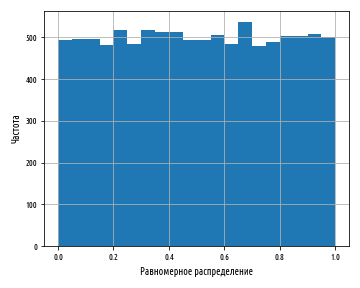
Каждый столбец гистограммы имеет примерно одинаковую высоту, что соответствует равновероятности генерирования числа, которое попадает в каждую корзину. Столбцы имеют не совсем одинаковую высоту, потому что равномерное распределение описывает теоретический результат, который наша случайная выборка не может отразить в точности. Раздел инференциальной статистики, посвященный проверке статистических гипотез, изучает способы точной количественной оценки расхождения между теорией и практикой, чтобы определить, являются ли расхождения достаточно большими, чтобы обратить на это внимание. В данном случае они таковыми не являются.
Если напротив сгенерировать гистограмму средних значений последовательностей чисел, то в результате получится распределение, которое выглядит совсем непохоже.
Приведенный выше пример сгенерирует результат, аналогичный следующей ниже гистограмме:
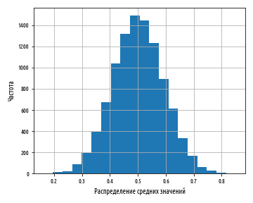
Хотя величина среднего значения близкая к 0 или 1 не является невозможной, она является чрезвычайно невероятной и становится менее вероятной по мере роста числа усредненных чисел и числа выборочных средних. Фактически, на выходе получается результат очень близкий к нормальному распределению.
Этот результат, когда средний эффект множества мелких случайных колебаний в итоге приводит к нормальному распределению, называется центральной предельной теоремой, иногда сокращенно ЦПТ, и играет важную роль для объяснения, почему нормальное распределение встречается так часто в природных явлениях.
До 20-ого века самого термина еще не существовало, хотя этот эффект был зафиксирован еще в 1733 г. французским математиком Абрахамом де Mуавром, который использовал нормальное распределение, чтобы аппроксимировать число орлов в результате бросания уравновешенной монеты. Исход бросков монеты лучше всего моделировать при помощи биномиального распределения. В отличие от центральной предельной теоремы, которая позволяет получать выборки из приближенно нормального распределения, библиотека scipy содержит функции для эффективного генерирования выборок из самых разнообразных статистических распределений, включая нормальное:
Отметим, что в функции sp.random.normal параметр loc – это среднее значение, scale – дисперсия и size – размер выборки. Приведенный выше пример сгенерирует следующую гистограмму нормального распределения:

По умолчанию среднее значение и стандартное отклонение для получения нормального распределения равны соответственно 0 и 1.
Примеры исходного кода для этого поста находятся в моем репо на Github. Все исходные данные взяты в репозитории автора книги.
Следующая часть, часть 3, серии постов «Python, исследование данных и выборы» посвящена генерированию распределений, их свойствам, а также графикам для их сопоставительного анализа